Online reader
RL without Tears
The online version follows the chapter structure of the paper, but it is written as a guided reading path rather than a compressed abstract. Each section answers the question left by the previous one: what an LLM policy is, how rewards can train it, why PPO-style RLHF needs stabilizers, and how the same feedback loop later extends to reasoning, agents, and multimodal models. The PDF remains the complete version for derivations, references, and detailed discussion.
Section 1
Introduction
Reinforcement learning is a framework for improving behavior from feedback. An agent makes decisions, receives signals from an environment, and adjusts its policy so that future decisions collect higher reward. Traditional introductions often begin with games, robotics, or control. This tutorial begins instead with LLMs: a model receives a prompt, generates a response token by token, and can be evaluated after the response or interaction is complete [1].
Why RL for LLMs?
The paper begins from a simple mismatch. Pre-training and supervised fine-tuning teach an LLM by showing it text to imitate, but many things we want from an assistant are easier to judge than to demonstrate exhaustively. Helpfulness, preference alignment, safety, reasoning correctness, and task success are often properties of a complete behavior, not properties of one isolated token. RLHF uses feedback over generated responses to align pretrained models with human preferences, while recent reasoning and agent systems extend the same idea toward learning from verifiers, tools, environments, and accumulated experience [3][2][12].
Intelligence, and its associated abilities, can be understood as subserving the maximisation of reward by an agent acting in its environment.
The Gap This Paper Fills
For NLP researchers, the difficulty is rarely the motivation. The difficulty is the translation layer. RL papers talk about states, actions, policies, trajectories, returns, critics, and advantages; LLM papers talk about prompts, tokens, log probabilities, completions, preference data, reward models, and KL penalties. The two vocabularies describe compatible objects, but they are often introduced from different examples. This tutorial fills that gap by keeping the mathematical language of RL while grounding each concept in an LLM training situation.
| Reader Question | How the Paper Answers It |
|---|---|
| How is an LLM a policy? | Map the prompt and generated prefix to a state, and the next token to an action. |
| Why use rewards instead of only demonstrations? | Rewards evaluate generated behavior when exact target outputs are hard to specify. |
| Why are value functions and advantages needed? | They reduce gradient variance and make policy optimization more stable. |
| Why do PPO, GRPO, and DPO matter? | They represent different ways to optimize policies from reward or preference feedback. |
Roadmap
The introduction then sets the scope of the paper. The tutorial proceeds in the order a reader needs the concepts. Section 2 first builds the shared notation: LLM generation is a sequence of decisions, and RL gives names to the decision process and feedback. Section 3 then turns that notation into a complete PPO-style RLHF workflow. Section 4 revisits the workflow and asks where it breaks or becomes expensive. Sections 5 to 7 apply the same lens to reasoning, agents, and multimodal models, where trajectories become longer, rewards become more varied, and credit assignment becomes more important.
Translate prompts, prefixes, tokens, and completions into states, actions, policies, and trajectories.
Use one LLM training example to derive the reward-scoring and policy-update loop.
Strengthen rewards, advantages, efficiency, and preference optimization after the basic loop is clear.
Follow the same feedback logic into reasoning, agents, and multimodal models.
Section 2
Preliminary: LLMs and RL
Before introducing policy gradients or PPO, the tutorial first makes the two sides of the story use the same language. On the LLM side, generation is a sequence of next-token decisions conditioned on a prompt and the prefix generated so far. On the RL side, learning is a sequence of decisions made by a policy, evaluated by rewards along a trajectory. Section 2 connects these views so that the later algorithms can be read as operations on familiar LLM objects.
The LLM review is intentionally selective. It covers the concepts that will later become RL variables: token probabilities, prompts, supervised fine-tuning, decoding, and sampled outputs. It is not meant to replace a full LLM survey; readers who want a broader background can refer to Foundations of Large Language Models.
2.1 Fundamentals of LLMs
Modern generative LLMs are usually decoder-only Transformers. A tokenizer first converts raw text into tokens from a vocabulary \(\mathcal{V}\), and the model assigns probability to a token sequence \(\mathbf{z}=z_1,\ldots,z_N\) by factorizing it from left to right. This factorization matters for RL: once a response is written as a product of next-token probabilities, changing the probability of a sampled response can be decomposed into changing the probabilities of the tokens that formed it.
Here, \(\mathbf{z}_{<i}=z_1,\ldots,z_{i-1}\) denotes the tokens before \(z_i\). Causal self-attention ensures that the prediction at each position only depends on previous tokens.
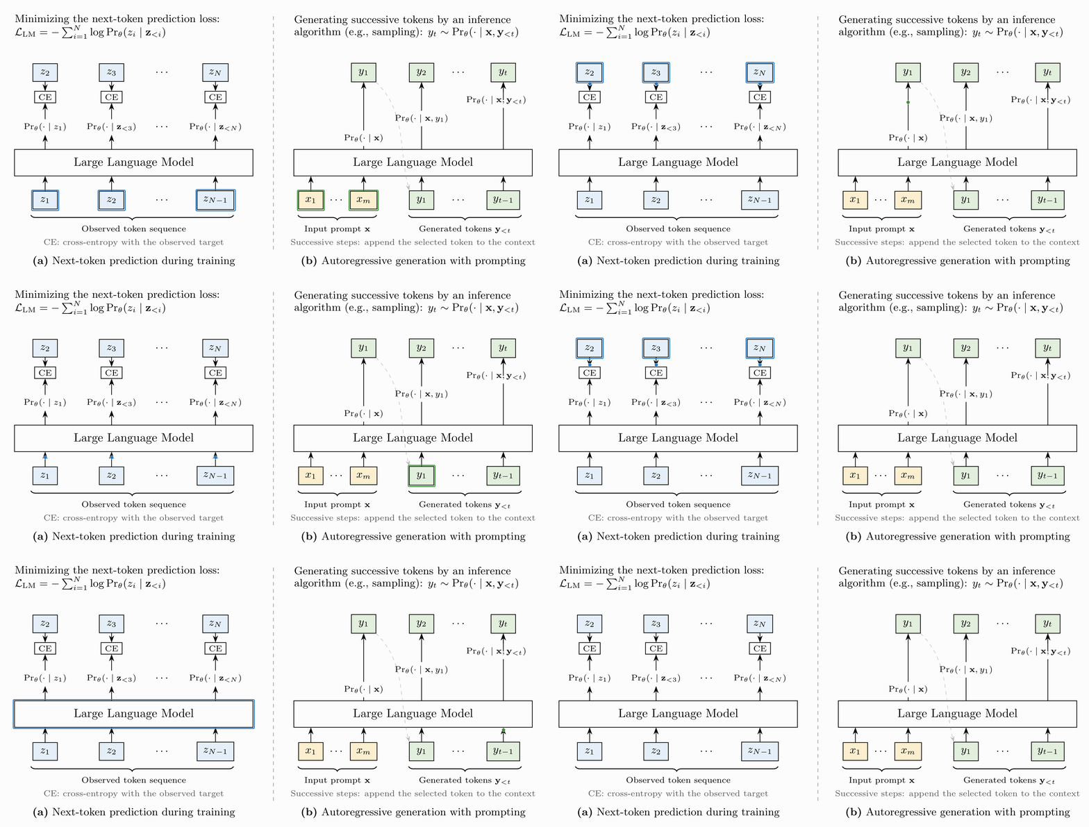
Pre-training
Pre-training teaches the model general language capabilities from large-scale unlabeled text. Each token in a corpus naturally becomes a self-supervised target: the model observes the preceding context and learns to predict the next token. If \(\mathcal{S}_{\mathrm{pre}}\) denotes the pre-training corpus, the objective maximizes the total log-likelihood of all tokens.
After this stage, the model can produce fluent continuations and has absorbed linguistic and factual regularities from data. However, the objective is still to model text, not to satisfy a user's current intention. That limitation motivates the next adaptation mechanisms: first change the input context with prompts, then change the model parameters with supervised fine-tuning, and later change behavior with reward-based learning.
Prompting
Prompting is a simple and lightweight way to adapt an LLM to different tasks without updating its parameters. A prompt is the input text used to guide the model toward a desired task or output. It may contain an instruction, user-provided content, output requirements, or demonstrations.
In this example, the prompt specifies both the task and the desired response style, and the LLM generates the answer by continuing the input sequence. Prompts can also be written as templates. For the same homework-assistant setting, we may keep the instruction fixed and replace only a task-specific placeholder:
If {subject} is replaced by "math", the template becomes the prompt above. If it is replaced by "English writing", the same instruction pattern is reused for a different task. This is why prompting is often the first adaptation method tried before any parameter update.
Another important concept related to prompting is in-context learning. By adding demonstrations to the context, we can let the model infer the desired input-output pattern from examples before responding to a new input.
When no demonstration is provided, the setting is usually called zero-shot prompting. When one demonstration is included, it is called one-shot prompting. When several demonstrations are included, it is called few-shot prompting. The key idea is that the model uses examples in the current context to infer the expected input-output pattern without changing its parameters.
In-context learning can also be combined with chain-of-thought (CoT) prompting. CoT prompting encourages the model to generate intermediate reasoning steps before giving the final answer. This can be done by directly asking the model to reason step by step or by providing demonstrations that include both the reasoning process and the answer.
Prompting adapts an LLM by changing the context used for generation. Therefore, prompt quality can strongly affect model performance. Even for the same task, we can write the prompt in many different ways. For example, "Give me two tips to improve my English writing." can also be written as "What are two simple ways to improve my English writing skills?". The two prompts express nearly the same intent, but they may lead to noticeably different outputs. Prompting is powerful because it is cheap, but it also exposes a limit: if the model does not reliably know the desired behavior, changing the context may not be enough. Supervised fine-tuning addresses this by updating the model on examples of desired responses.
Supervised Fine-Tuning
Supervised fine-tuning further adapts a pretrained model using labeled input-output pairs. The input \(\mathbf{x}\) typically combines an instruction and user content, while the output \(\mathbf{y}\) is the desired response. SFT teaches the model both what knowledge to express and how to express it in an instruction-following format.
| Task | Input | Output |
|---|---|---|
| Summarization | Summarize an article about rapid growth in solar energy. | Solar energy has grown rapidly and become a major renewable source. |
| Question answering | What is the capital of France? | Paris. |
| Classification | Classify a prize-message as spam or not spam. | Spam. |
| Machine translation | Translate "RL is widely used to train LLMs" into Chinese. | 强化学习被广泛用于训练大语言模型。 |
Here, \(\mathcal{S}\) denotes the labeled data, \(\tilde{\theta}\) denotes the parameters optimized via SFT, and \(\hat{\theta}^{+}\) represents an adjustment to the pretrained parameters \(\hat{\theta}\). The fine-tuning starts from the pretrained parameters rather than randomly initialized ones.
This formulation is equivalent to minimizing the cross-entropy loss over the output segment. In practice, the input tokens are used as context and the loss is usually computed only on the output tokens. The resulting SFT model is often the starting policy for later RL training: it can already follow the task format, but it may still need feedback to prefer one acceptable response over another.
Inference
Inference applies the trained LLM to new inputs. Given a prompt \(\mathbf{x}\), the model predicts a distribution over the first output token, selects a token with a decoding strategy, appends it to the context, and repeats this autoregressive process until a stopping condition is reached.
| Decoding Strategy | How It Selects the Next Token | Tradeoff |
|---|---|---|
| Greedy decoding | Selects the highest-probability token at each step. | Fast and deterministic, but locally optimal choices may hurt the full sequence. |
| Beam search | Keeps the top \(B\) candidate prefixes and expands them step by step. | Explores more candidates, but costs more compute and memory. |
| Sampling | Samples from \(\mathrm{Pr}_{\theta}(\cdot\mid\mathbf{x},\mathbf{y}_{<t})\), often with temperature, top-\(k\), or top-\(p\) filtering. | Produces diverse outputs and closely resembles stochastic policy sampling in RL. |
This token-by-token generation view is the key bridge to RL. At timestep \(t\), the current context \((\mathbf{x},\mathbf{y}_{<t})\) can be treated as the state, the selected token \(y_t\) as the action, and the model distribution as the policy. Sampling is especially important because it produces the candidate trajectories that later receive rewards.
2.2 Fundamentals of RL
With the LLM side in place, the RL side becomes easier to read. RL provides a framework for learning from feedback: an agent observes a state, selects an action according to a policy, receives a reward, and transitions to a new state. For LLMs, this is most useful when exact demonstrations are hard to specify but generated behavior can still be judged by humans, reward models, rules, verifiers, or environments.

This interaction process is commonly modeled as a Markov Decision Process. A trajectory is a sequence of states and actions, \(\tau=(s_0,a_0,s_1,a_1,\ldots,s_{H-1},a_{H-1})\), whose quality is evaluated by accumulated rewards. The objective is to learn a policy that maximizes expected cumulative reward.
In LLM training, sampling means generating one or more trajectories from the current policy. A trajectory may be a completion, a reasoning trace, a tool-use interaction, or a multimodal generation path. Once the trajectory receives feedback, RL algorithms update the policy to make better behavior more likely.
| Element | Interpretation |
|---|---|
| Agent | The learner or decision-maker in RL. In the context of LLMs, the agent corresponds to the language model itself, which generates tokens sequentially and updates its behavior based on feedback signals. |
| Environment | Everything external to the agent with which it interacts. Unlike traditional RL settings that involve physical or simulated environments, the environment in LLM-based RL is typically abstract, consisting of the training framework that provides feedback, such as reward models, human annotations, or evaluation metrics, for generated outputs. |
| State \((s)\) | A state represents the current situation of the environment. For language modeling, the state at timestep \(t\) can be defined as the sequence of observed tokens up to that point, namely the context used to predict the next token. Formally, \(s_t=(\mathbf{x},\mathbf{y}_{<t})\), where \(\mathbf{x}\) denotes the input prompt and \(\mathbf{y}_{<t}\) denotes the previously generated tokens. |
| Action \((a)\) | An action corresponds to a decision made by the agent. In LLMs, actions are naturally defined as selecting the next token from the vocabulary, i.e., \(a_t=y_t\). |
| Reward \((r)\) | The reward provides feedback from the environment to evaluate the quality of an action. In general, the reward function can be defined as \(r(s,a,s')\), representing the feedback received when the agent transitions from state \(s\) to \(s'\) by taking action \(a\). At timestep \(t\), this can be written as \(r_t=r(s_t,a_t,s_{t+1})\). In deterministic settings, where the next state is uniquely determined by \((s_t,a_t)\), the reward can be simplified as \(r(s_t,a_t)\). |
| Policy \((\pi)\) | The policy defines the agent's behavior, i.e., the probability of taking an action given a state. For LLMs, the policy corresponds to the conditional probability distribution over the next token given the context: \(\pi_{\theta}(a_t\mid s_t)=\mathrm{Pr}_{\theta}(y_t\mid\mathbf{x},\mathbf{y}_{<t})\), where \(a_t=y_t\) and \(s_t=(\mathbf{x},\mathbf{y}_{<t})\). Under this formulation, an LLM can be naturally interpreted as a parameterized policy. |
| Value Function \((V\) and \(Q)\) |
The value function estimates the expected cumulative reward when following a policy. The state-value function \(V(s)\) measures the expected discounted return starting from state \(s\), while the action-value function \(Q(s,a)\) further conditions on the initial action. |
These correspondences let the rest of the tutorial describe RL algorithms using familiar language-model objects: contexts, tokens, log probabilities, rewards, values, and sampled outputs.
Section 3
Understanding RL in LLM Training
After Section 2 maps LLM generation into RL notation, Section 3 shows how the machinery works in an actual LLM training setting. The running example is a homework assistant whose SFT response is correct but too short. This is a useful example because the desired improvement is easy to judge but awkward to specify as a single gold answer. Rather than writing many new demonstrations, the tutorial defines feedback over generated outputs and uses RL to make preferred behavior more likely.
The section develops the workflow in dependency order. Policy gradient explains how a scalar reward can update a stochastic language model. Temporal decomposition explains how a response-level reward touches token-level decisions. Baselines and advantages reduce noisy updates. Importance sampling and PPO make repeated updates from sampled data more stable. Reward modeling then replaces hand-written feedback with learned preference scores, and the pieces finally assemble into the standard PPO-based RLHF loop.
Generate outputs from the policy.
Evaluate outputs with rewards.
Compute values or advantages.
Optimize the policy with PPO-style constraints.
3.1 Policy Gradient
Policy gradient methods answer the first training question: if we can only score completed samples, how can we update the model that produced them? In LLM training, the policy is the conditional distribution over generated tokens. Since it is impossible to enumerate all possible outputs, the expected reward is estimated with sampled responses.
From the paper's LLM notation
Because the hypothesis space \(\Omega\) is too large to enumerate, the paper approximates it with sampled outputs \(\mathcal{D}=\{\mathbf{y}_1,\ldots,\mathbf{y}_d\}\).
Here, \(J(\theta)\) denotes the policy objective, \(\pi_{\theta}\) is the policy model parameterized by \(\theta\), and \(\tau\) denotes a sampled trajectory. \(R(\tau)\) is the cumulative reward assigned to the trajectory, while \(\nabla_{\theta}\log \pi_{\theta}(\tau)\) gives the gradient of the trajectory log probability under the current policy.
The policy-gradient form is useful because the reward itself does not need to be differentiable. The reward may be provided by a human annotator, a learned reward model, a rule-based checker, or an external environment. The model update only requires the log probability of the sampled trajectory under the current policy [1].
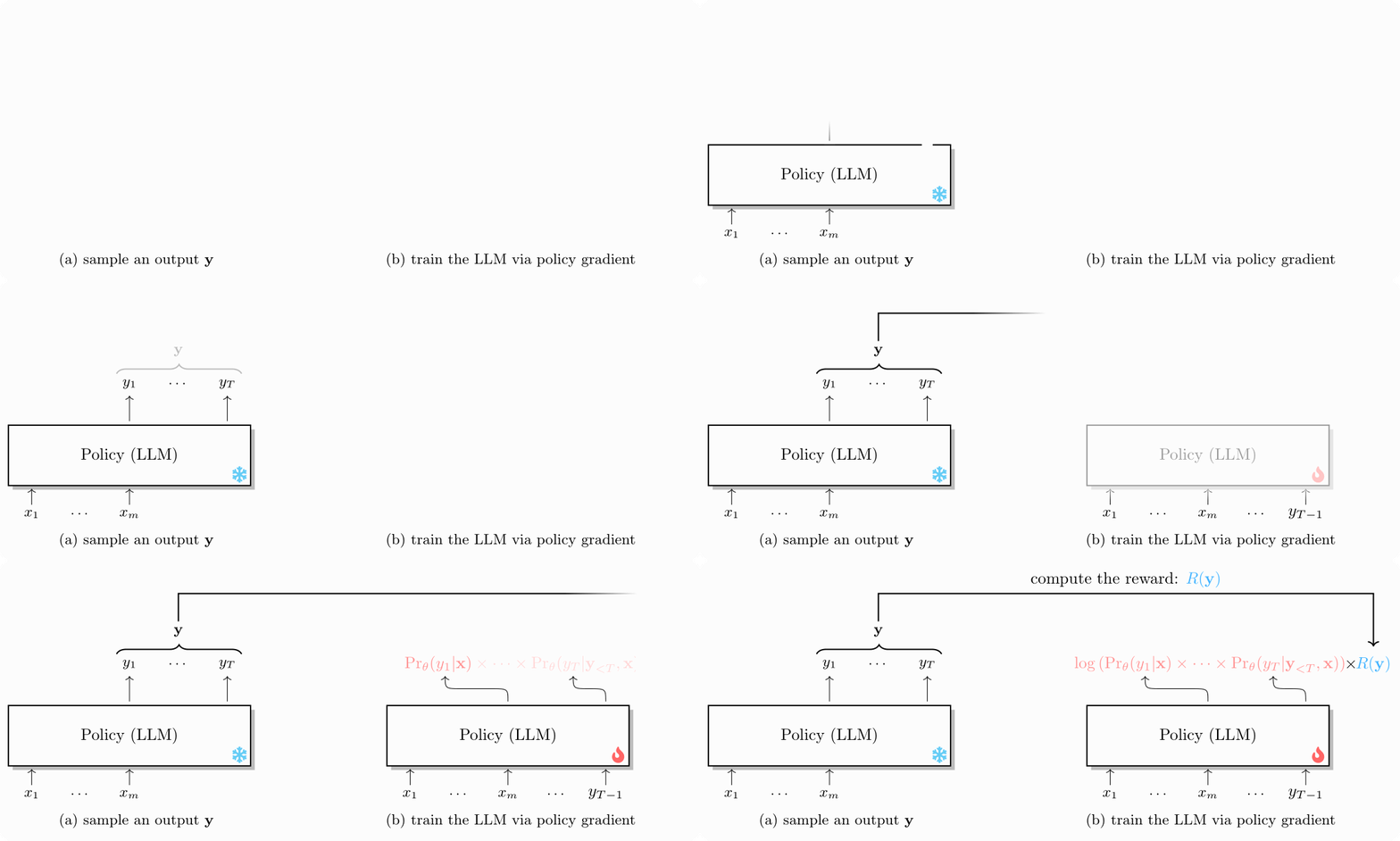
Thus, sampled responses with higher rewards are assigned higher probability, while responses with lower rewards are assigned lower probability. The following subsections refine this basic policy-gradient principle to handle long sequences, noisy rewards, and unstable updates.
3.2 Temporal Decomposition
The basic policy-gradient expression scores a whole response, but an LLM is updated through token probabilities. Temporal decomposition connects these levels. Because a generated response is composed of tokens, the probability of the full response can be decomposed into token-level probabilities, allowing a sequence-level reward to affect the individual decisions that produced the sequence.
Time-step decomposition from the paper
At the \(t\)-th generation step, \(y_t\) does not affect the past-reward term \(\sum_{k=1}^{t-1}r_k\). The paper therefore removes that term and keeps the future return from \(t\) onward.
The difficulty is that sequence-level rewards do not directly tell us which token caused success or failure. A correct answer may contain many ordinary tokens that are not responsible for the reward. An incorrect answer may be wrong because of one early reasoning error. Thus, temporal decomposition gives a mathematical path for training, but it does not fully solve credit assignment.
This issue becomes more important as outputs become longer. In short answers, assigning the same reward to all tokens may be acceptable. In reasoning traces and agent trajectories, a single final reward is too coarse. Later sections therefore discuss process rewards, verifiers, and agentic credit assignment.
3.3 Reducing Gradient Variance
Temporal decomposition gives every token a learning signal, but that signal can be very noisy. Directly using raw rewards may increase the probability of actions simply because they appeared in a generally good trajectory, even if those actions were not better than usual for the current state. To reduce this variance, policy-gradient methods introduce baselines and advantages.
Here, \(A(s,a)\) denotes the advantage of taking action \(a\) at state \(s\). \(Q(s,a)\) denotes the expected return after first taking action \(a\) at state \(s\), and \(V(s)\) denotes the expected return from state \(s\) under the policy.
The advantage measures whether an action is better than the expected behavior at the same state. A value model estimates the expected future reward. Subtracting this baseline keeps the expected gradient correct while making the update more stable.
In LLMs, value models are often implemented by reusing a pretrained backbone and adding a scalar head. They resemble reward models architecturally, but their function is different. A reward model evaluates an output. A value model estimates the expected return of a state under the current policy.
| Model | Role in PPO-style RLHF | Updated? |
|---|---|---|
| Policy model | Generates outputs and receives policy-gradient updates. | Yes. |
| Reward model | Scores generated outputs using learned preference signals. | Usually fixed during policy optimization. |
| Value model | Predicts expected return to estimate advantages. | Yes. |
| Reference model | Regularizes the policy and limits excessive drift. | No. |
3.4 Importance Sampling
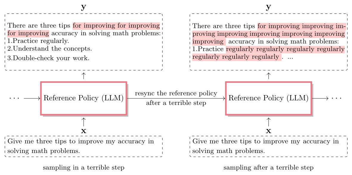
Once advantages make the update less noisy, another practical issue appears: the data may already be a little stale. Sampled outputs are often generated by an older version of the policy, while optimization happens after one or more parameter updates. Importance sampling corrects this mismatch by using the probability ratio between the current policy and the old policy.
Here, \(\rho_t(\theta)\) denotes the importance sampling ratio at timestep \(t\). \(\pi_{\theta}\) is the current policy, \(\pi_{\theta_{\mathrm{old}}}\) is the old policy that generated the sampled action, \(s_t\) is the state, and \(a_t\) is the action taken at that state.
This ratio is necessary because data freshness matters. If the learner updates too far from the policy that produced the samples, the samples become less reliable. The paper illustrates this with a poor sampling step that can make subsequent generations worse if the reference policy is not controlled.
3.5 Proximal Policy Optimization
Importance sampling tells the optimizer how much the current policy differs from the policy that produced the sample. PPO adds a guardrail around that difference. Its main idea is to prevent the policy from changing too much in a single update by clipping the importance ratio in the objective function [4].
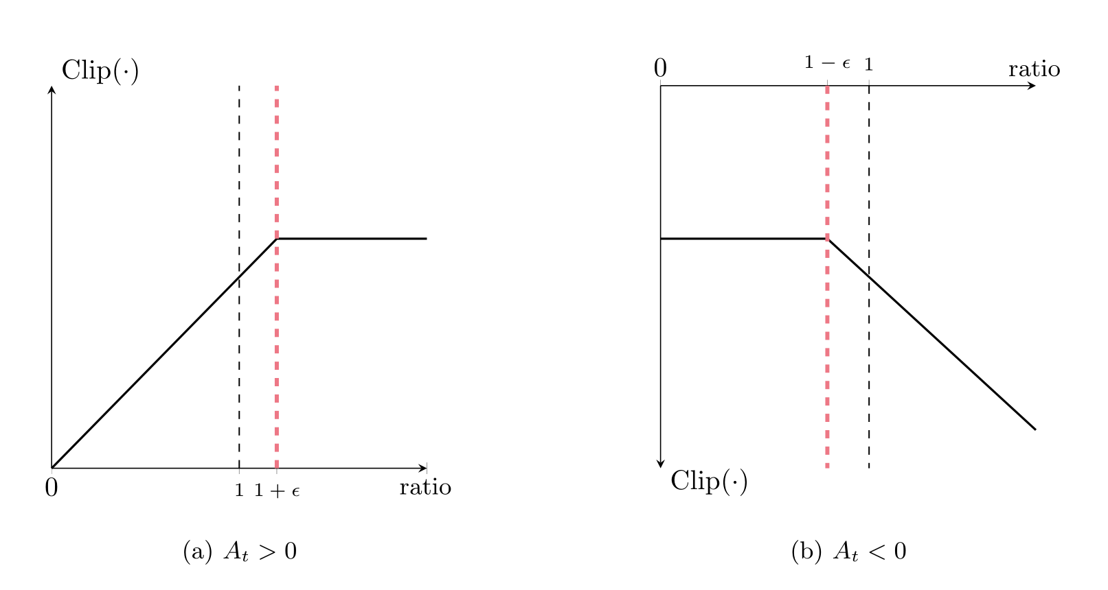
Here, \(\rho_t\) is the probability ratio between the current and old policies, and \(A_t\) is the advantage estimated at timestep \(t\). The clipping range \([1-\epsilon,1+\epsilon]\) limits how much the policy can change in one update.
If the advantage is positive, the model is encouraged to increase the probability of the action, but only within a bounded range. If the advantage is negative, the model is encouraged to reduce the probability, again with a limit. This makes PPO suitable for RLHF, where excessive reward optimization can damage language quality or exploit weaknesses in the reward model.
This is the paper's PPO loss: the clipped advantage term updates the policy, while \(\beta \mathrm{Penalty}_t\) constrains drift from the reference model.
3.6 Training Reward Models
Up to this point, the reward can be imagined as a simple score. RLHF needs a scalable way to produce that score for many sampled responses, so it usually trains a reward model before policy optimization. A reward model maps an input-output pair to a scalar score and is commonly trained from pairwise preference data, where a human or AI judge chooses the better response among two candidates [5].
The paper first describes several ways to collect feedback. Rating asks annotators to assign numerical scores. Listwise ranking asks them to order a set of candidate outputs. Pairwise comparison asks them to choose the better of two outputs for the same input. Pairwise comparison is widely used because it is usually easier and more reliable than assigning absolute scores.
Here, \(\mathcal{L}_{\mathrm{RM}}\) denotes the reward model loss, \(r_{\phi}\) is the reward model parameterized by \(\phi\), \(\mathbf{x}\) is the input, \(\mathbf{y}_w\) is the preferred output sequence, and \(\mathbf{y}_l\) is the rejected output sequence. The sigmoid function turns the reward difference into a preference probability.
Pairwise comparison is commonly used because it is often more reliable to annotate than absolute numerical scores. Once trained, the reward model can score many newly generated responses, providing a scalable signal for policy optimization.

During policy optimization, the reward model usually scores a complete input-output pair independently. This means the reward is often sparse: intermediate tokens receive no direct reward, and the final token receives the reward model score. This limitation is one reason later sections discuss reward shaping, process reward models, and step-level verification.
3.7 A Complete Workflow
The section concludes by combining the components into a standard PPO-based RLHF workflow. First, a reward model is trained from preference data. Then the policy samples outputs. The reward model scores these outputs, a value model estimates advantages, and PPO updates the policy under a reference policy constraint.

This workflow explains why RLHF is not only an algorithmic objective. It is a training system involving data generation, reward inference, KL regularization, advantage estimation, optimization, and evaluation. Once the system view is clear, the next chapter becomes natural: many modern methods can be understood as attempts to make one component of this loop more reliable, cheaper, or easier to optimize [2].
Section 4
Improved RL for LLMs
Section 3 builds the basic PPO-style RLHF workflow. Section 4 keeps the same workflow in view and asks what must be improved before it becomes practical at modern LLM scale. The discussion is organized around four pressure points: how to construct better rewards, how to estimate advantages without excessive variance or cost, how to spend less computation during online training, and when to replace the explicit reward-model-plus-RL pipeline with direct preference learning.
| Problem | Methods Discussed | Main Benefit |
|---|---|---|
| Sparse or weak rewards | Reward shaping, rule-based rewards, process rewards. | Provides denser or more reliable feedback. |
| Reward model limitations | Generative reward models, rubric-based rewards, reward evaluation. | Improves alignment and evaluation transparency. |
| Expensive or unstable critics | TD, GAE, GRPO, value-free advantage estimation. | Improves the bias-variance and system-cost tradeoff. |
| Pipeline complexity | DPO and related direct preference methods. | Optimizes from preference pairs without an explicit online RL loop. |
The order of the chapter mirrors the training loop. It starts with the reward because the reward defines what the policy will learn. It then moves to advantage estimation because rewards must be converted into stable token-level updates. Efficiency comes next because sampling and scoring dominate practical cost. DPO is discussed last because it changes the pipeline itself.
4.1 Advanced Reward Models
Reward construction strongly determines what the policy learns. If the reward is sparse, noisy, biased, or vulnerable to exploitation, policy optimization may produce behavior that scores well without matching the true objective. Therefore, modern LLM RL places increasing emphasis on reward design.
4.1.1 Automatic Preference Data Generation
The first issue is data. Human preference labels are useful, but they are expensive and subjective. A scalable alternative is to ask a strong model or verifier to compare candidate outputs. In the homework-assistant example from the paper, the judge sees the input and two candidate answers, then selects the one that is more informative, accurate, clear, and helpful.
This makes preference data easier to scale because the system can generate both outputs and labels. However, the paper also stresses the risk: AI feedback can inherit position bias, judge-specific preferences, and mistakes in the judging prompt. In practice, prompt design, demonstrations, diverse candidate generation, and mixing human and AI feedback are used to improve the quality and diversity of generated preference data.
4.1.2 Reward Shaping
The second issue is sparsity. A standard reward model often gives only one score after the entire response is generated. This delayed reward is difficult to assign back to individual token decisions, especially for long reasoning traces or agent trajectories. Reward shaping addresses this by adding intermediate rewards that make the learning signal denser.
For example, an LLM can receive a delayed reward from a reward model at the end of the answer, while also receiving intermediate rewards for valid formatting, correct intermediate reasoning, or useful partial progress. The paper connects this idea to potential-based shaping:
When the potential function is a value function, this form becomes closely related to advantage estimation. The important caveat is that shaping rewards must remain aligned with the final objective. Otherwise the model may optimize the intermediate signal instead of the behavior we actually want.
4.1.3 Improved Reward Generalization
The third issue is generalization. During RL, the policy changes and begins to generate outputs that may differ from the preference data used to train the reward model. A reward model that works well on a static validation set may still fail when the policy learns to exploit its weaknesses.
This failure mode is often called reward hacking or overoptimization: the reward model score improves, but the real quality of the model's behavior does not. The paper discusses several practical defenses. Ensembles combine multiple reward models to reduce single-model errors. Parameter freezing and regularization help preserve the general features of the underlying LLM. More diverse preference data reduces the chance that the reward model only works on a narrow distribution.
4.1.4 Generative Reward Models
Conventional reward models usually assign scalar scores to outputs. Generative reward models instead formulate preference judgment as a language modeling task. The model receives the prompt, input, and candidate outputs, and generates a label or judgment token [6].
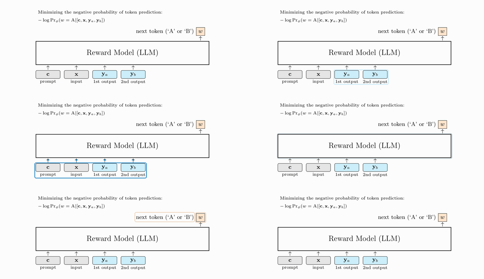
This formulation can leverage the reasoning ability and instruction-following behavior of LLMs. It is especially useful when evaluation requires comparing responses with nuanced criteria rather than only assigning an independent scalar score.
4.1.5 Rubric-based Reward Models
Rubric-based reward models make evaluation criteria explicit. Instead of asking for a single opaque preference, a rubric specifies dimensions such as correctness, completeness, instruction following, safety, style, and evidence. The reward model then evaluates responses according to these criteria.
Rubrics can be holistic, criterion-wise, checklist-based, or hierarchical. A holistic rubric gives an overall judgment based on several criteria. A criterion-wise rubric scores each dimension separately. A checklist rubric decomposes evaluation into atomic conditions. A hierarchical rubric organizes criteria across multiple levels.
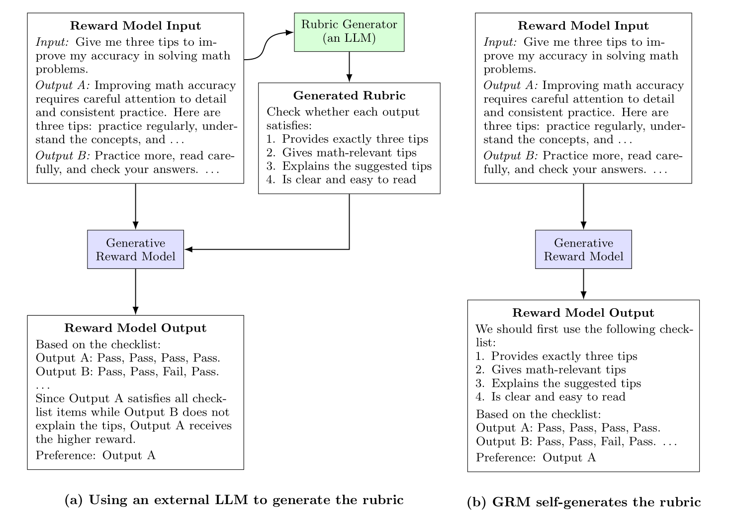
Rubric generation can be manual or automatic. Automatic rubric generation is attractive because it adapts evaluation criteria to each input. The paper also discusses rubric optimization, where rubrics are refined through preference data or RL so that they better distinguish high-quality responses [7].
4.1.6 Reward Model Evaluation
Evaluating reward models is difficult because a reward model is not the final application. It is used to train or select policies. A reward model may perform well on static preference prediction but still fail when a policy learns to exploit it during optimization.
The paper summarizes three evaluation paradigms. RL-based evaluation uses each reward model to train a policy and compares the resulting policies on downstream benchmarks. Pairwise ranking evaluation checks whether the reward model assigns a higher score to the preferred response. Listwise ranking evaluation asks the reward model to select the best response from multiple candidates [8].
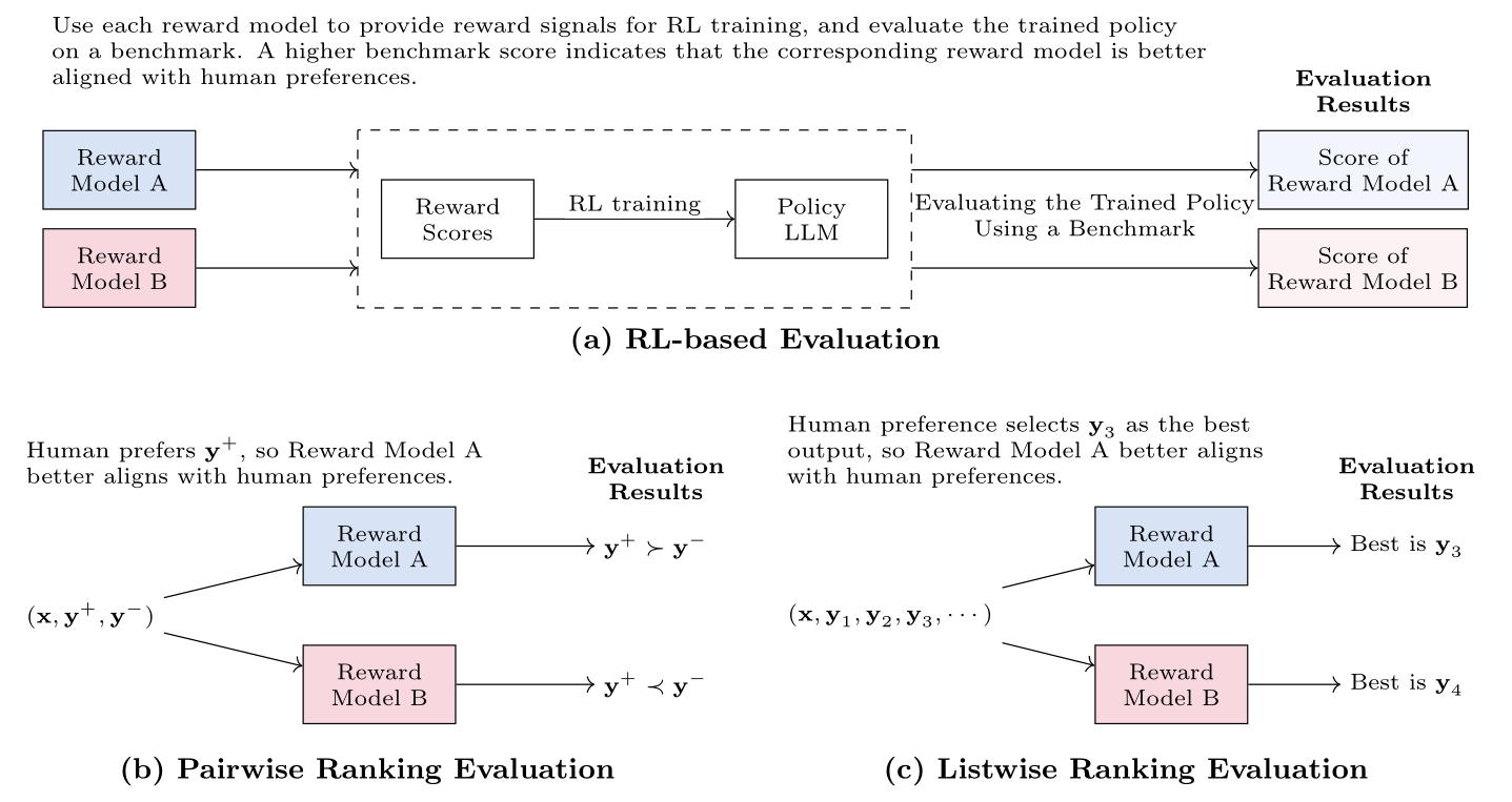
These evaluations answer different questions. Pairwise and listwise ranking are more efficient to scale. RL-based evaluation is more expensive, but it measures the reward model in the setting where it will actually be used. In practice, both static and downstream evaluations are useful.
4.2 Better Advantage Estimation
After improving reward construction, the next question is how to turn those rewards into policy updates. Advantage estimation balances bias and variance in policy optimization. Monte Carlo estimates can be less biased because they use observed returns, but they often have high variance. Temporal-difference methods reduce variance by bootstrapping from value estimates, but they may introduce bias.
4.2.1 Temporal Difference-based Advantage Estimation
The basic Monte Carlo advantage in Section 3 uses the observed future return minus a value baseline. This is intuitive, but long LLM outputs make the observed return noisy. Temporal-difference estimation replaces a full future return with a one-step target: immediate reward plus the value of the next state. This makes the estimate less noisy because it bootstraps from the value model instead of waiting for the whole trajectory.
Here, \(\delta_t\) is the temporal-difference residual. It measures whether the observed transition was better or worse than the value model expected.
The tradeoff is bias: if the value model is inaccurate, the bootstrapped target can be wrong. This is why advantage estimation is usually presented as a bias-variance problem rather than a single best formula.
4.2.2 Generalized Advantage Estimation
Generalized advantage estimation combines these ideas through a tunable tradeoff. In LLM training, the problem is complicated by long sequences and delayed rewards. A separate critic can estimate token-level values, but training a reliable critic for language can be expensive and unstable [9].
\(\lambda\) controls how much future temporal-difference information is mixed into the current advantage. Smaller values rely more on short-horizon bootstrapping; larger values behave more like Monte Carlo returns.
4.2.3 Group Relative Policy Optimization
GRPO addresses the cost and instability of a separate critic by estimating advantages from a group of responses sampled for the same prompt. Instead of relying on a learned value model, it normalizes rewards within the group. A response is considered good if it performs better than other sampled responses to the same input [10].

Here, \(G\) is the number of sampled outputs in the group, and \(A_{i,t}^{\mathrm{GRPO}}\) is the group-relative advantage used for the \(i\)-th output.
This method is well suited to reasoning tasks, where multiple candidate solutions can be generated and scored by a verifier. The group provides a natural baseline. Removing the critic can simplify training and reduce computational cost.
| Estimator | Uses | Tradeoff |
|---|---|---|
| Monte Carlo | Observed complete returns. | Low bias, high variance. |
| Temporal Difference | Immediate reward plus next value. | Lower variance, possible bias. |
| GAE | Recursive TD errors with gamma and lambda. | Adjustable bias-variance balance. |
| GRPO | Relative rewards within a sampled group. | Avoids a separate value model. |
4.3 Efficient RL Methods
Even with better rewards and advantages, RL post-training remains expensive. The cost is not only the optimizer step. A training loop must repeatedly generate rollouts, score them, estimate advantages, update the policy, and often keep several models in memory at the same time. For LLMs, this becomes a time-efficiency problem and a space-efficiency problem: we want to reach the desired RL performance with less wall-clock time, fewer sampled tokens, fewer reward-model calls, and lower memory pressure.
This section focuses on two practical sources of waste. The first is sampling. Every prompt in the RL dataset may require autoregressive generation, and large-scale RL can repeat this process for many training steps. The second is reward computation. A reliable reward model may itself be a large LLM, so scoring every rollout can be expensive. Efficient RL methods therefore ask a simple question: which parts of the loop are truly needed for learning, and which parts can be skipped, approximated, or replaced with cheaper signals?
| Cost Source | Why It Is Expensive | Efficiency Strategy |
|---|---|---|
| Rollout sampling | The policy must generate tokens autoregressively before rewards are available. | Use inference acceleration or sample only prompts that need exploration. |
| Reward scoring | Large reward models add extra forward passes for every sampled output. | Use rules, verifiers, smaller reward models, distillation, pruning, or mixture-of-experts designs. |
| Auxiliary models | PPO-style training may keep policy, reference, reward, and value models active. | Remove or simplify components when possible, as in value-free advantage methods or direct preference methods. |
| Uninformative prompts | Some prompts are already solved, while others are too hard at the current stage. | Prioritize prompts whose rewards indicate room for useful improvement. |
4.3.1 Dynamic Sampling
Sampling is one of the main costs of RL for LLMs because the policy must autoregressively generate outputs before they can be scored. Dynamic sampling asks whether every prompt really needs the same amount of exploration. If the current policy already gives a high-reward answer to a prompt, further sampling may be wasteful. If a prompt is too difficult and consistently receives very low rewards, repeated exploration may also be inefficient.
From the inference side, many standard LLM acceleration techniques can reduce rollout time, such as KV caching, quantization, batching, and speculative decoding. Dynamic sampling is different: it reduces sampling from the RL training side by deciding which prompts deserve exploration in the first place. The motivation is that an SFT or pretrained policy is not a randomly initialized agent. For some prompts, it already produces a strong answer; for others, the current policy may be too weak to discover a useful trajectory without much more capability. Treating both cases equally wastes sampling budget.
A simple strategy is to first generate a greedy answer \(\hat{\mathbf{y}}_k\) for each prompt \(\mathbf{x}_k\), then score that answer with a reward model:
Here, \(R_k\) is the reward assigned to the current greedy output, \(N\) is the number of prompts in the input-only dataset \(\mathcal{S}_x\), and \(r_{\mathrm{upper}}\) is one possible upper threshold.
Prompts above the upper threshold can be skipped or sampled less often because the current policy is already doing well. A lower threshold \(r_{\mathrm{lower}}\) can also be introduced. Prompts below this lower threshold may be deprioritized because the policy is unlikely to find a useful output at the current stage. The most valuable prompts often lie between the two thresholds:
This middle region is where exploration is most likely to pay off. The model is not already perfect, but it is also not completely lost. Sampling multiple rollouts for these prompts can expose meaningful reward differences, which gives PPO, GRPO, or other RL optimizers a stronger learning signal per token generated.
The tradeoff is that the thresholds become part of the training design. If \(r_{\mathrm{upper}}\) is too low, the method may stop training on prompts that still have room to improve. If \(r_{\mathrm{lower}}\) is too high, it may discard hard examples too aggressively and reduce robustness. In practice, dynamic sampling is often combined with periodic rescoring so that prompts can re-enter or leave the active set as the policy improves.
4.3.2 Lightweight Reward Methods
The second major cost is reward computation. In a standard RLHF loop, every sampled output must be passed to a reward model. If the reward model is large, this adds substantial inference cost on top of policy generation. Lightweight reward methods try to reduce that cost by replacing, complementing, or compressing the reward model.
Rule-based rewards are the clearest example. A math task can reward the correct final answer; a code task can reward passing tests; a formatting task can reward valid JSON with required fields. These rewards are fast, deterministic, and less vulnerable to reward-model miscalibration. They are especially useful in math, coding, formatting, and tool-use tasks, where correctness can sometimes be checked automatically.
| Reward Type | Example | Strength | Limitation |
|---|---|---|---|
| Format rule | Reward valid JSON containing required keys such as tip1, tip2, and tip3. | Cheap and exact. | Checks form, not necessarily substance. |
| Answer rule | Reward a math response if the final answer matches the verified solution. | Reliable when answers are checkable. | Can be sparse and may miss reasoning quality. |
| Execution verifier | Reward code that passes unit tests or a tool call that reaches the correct environment state. | Measures real task success. | Requires a trustworthy execution environment. |
| Small reward model | Distill or prune a larger reward model for faster scoring. | Keeps some flexibility of learned preference judgment. | May inherit errors or lose nuance. |
The main benefit of rules is stability. Because the reward is predefined, the policy cannot exploit hidden quirks of a learned reward model in the same way. However, rule-based rewards only work when the target behavior can be described by reliable checks. A JSON validity reward can enforce structure, but it cannot guarantee that the tips are actually useful. A final-answer reward can verify correctness, but it may not explain which reasoning step went wrong. This is why lightweight rewards are often strongest when combined with process rewards, verifiers, or occasional learned reward-model checks.
For broader preference alignment, learned reward models are still useful because the desired behavior is often too nuanced for simple rules. In that case, efficiency can come from making the reward model cheaper rather than removing it. Distillation can train a smaller reward model to imitate a larger one. Pruning and quantization can reduce inference cost. Mixture-of-experts reward models can activate only part of the model for each example. These approaches preserve more flexibility than hand-written rules, but they still require evaluation because a cheaper reward model may be less calibrated or less robust.
4.4 Direct Preference Optimization
The chapter ends with a method that changes the workflow more fundamentally. DPO offers a different approach to preference learning: instead of training a reward model and then applying RL, it optimizes the policy directly from preference pairs. This makes training closer to supervised learning and removes the need for an explicit online RL loop in the basic formulation [11].
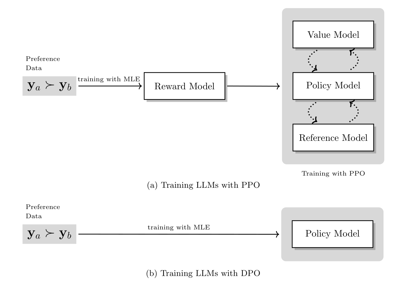
DPO simplifies the pipeline and is often more straightforward to implement. However, it is usually based on fixed preference data, while RL methods can continue sampling from the current policy and learning from newly generated behavior. PPO-style RL and DPO-style preference optimization therefore represent different tradeoffs between exploration, simplicity, and system cost.
Section 5
RL for LLM Reasoning
After the tutorial explains general RL training and its improvements, it turns to reasoning. This is the first major application chapter because reasoning makes the value of feedback especially visible. A math answer can be checked, code can be executed against tests, and tool-integrated reasoning can be evaluated through external results. These signals are often sparse, but they are more objective than open-ended preference judgments [12].
The section starts at test time because search and verification can improve answers before any parameter update. That gives the reader the basic pattern: generate multiple reasoning paths, evaluate them, and select or improve the best ones. The rest of the section then turns this inference-time pattern into training through iterative RL, large-scale RL, and on-policy distillation, so better reasoning becomes part of the model rather than only a procedure wrapped around it.
5.1 Test-time Scaling
Test-time scaling improves performance by generating multiple candidate reasoning paths and selecting a strong one. Best-of-N sampling is a representative example. The model samples several responses, a reward model or verifier scores them, and the highest-scoring response is returned.
This section starts with inference rather than training because reasoning quality often improves simply by spending more computation at test time. A prompt such as "Let's think step by step" can encourage longer reasoning, but it does not tell the model which reasoning path is actually better. Test-time scaling adds a selection signal: generate alternatives, evaluate them, and keep the most promising one.

In Best-of-N sampling, the candidates can be reranked by a reward model. If no reward model is available, majority voting can be used when answers are easy to compare, such as math problems with a final numeric result. The same idea can also be used for training through rejection sampling: sample multiple answers, keep the best ones, and fine-tune the model on those selected outputs.
This creates the bridge to RL. If a verifier can reliably identify better candidates at inference time, then the same signal can be used during training so that the model learns to generate strong reasoning paths more often without relying on many samples at test time.
5.1.2 Step-by-step Verification
Final-answer rewards may be too sparse for long reasoning chains. Step-by-step verification provides denser feedback by evaluating intermediate reasoning steps. This helps identify where a solution path begins to fail and supports more precise credit assignment [13].
Process reward models can score partial solutions, while greedy or beam-style procedures can extend the most promising paths. This shifts reasoning from one-shot generation toward guided construction of a solution.
The key change is the granularity of feedback. Instead of scoring only the final answer, the verifier scores each intermediate step or prefix. A path can then be abandoned early if its partial reasoning becomes unpromising. The same process reward can later serve as a shaping reward during RL, giving the model more informative feedback than a single outcome score.

5.1.3 Monte Carlo Tree Search
Monte Carlo Tree Search further formalizes reasoning as search. Nodes represent partial reasoning states, and edges represent candidate next steps. The search process selects promising nodes, expands them, simulates continuations, and backpropagates evaluation results [14].

MCTS is useful when the model has enough local reasoning ability to propose candidate steps, but needs search to find a reliable global solution. The verifier or reward model guides the search toward paths with higher expected success.
In the tutorial's framing, MCTS also clarifies why reasoning resembles sequential decision-making. Each reasoning step changes the state, future steps depend on earlier choices, and delayed rewards from a simulated final answer can be propagated back to earlier partial states.
| Test-time Method | Object Scored | Feedback Granularity |
|---|---|---|
| Best-of-N | Complete sampled outputs. | Outcome-level. |
| Step-by-step verification | Intermediate reasoning steps. | Process-level. |
| MCTS | Partial reasoning states and continuations. | Hybrid search feedback. |
5.2 Iterative RL
Once verifiers can identify better reasoning paths, the next question is how to turn that signal into a training recipe. Iterative RL is presented through the DeepSeek-R1 process. Instead of using a simple two-phase SFT-then-RL pipeline, the process is split into several phases with different objectives, so the model can improve reasoning ability while preserving readable and useful behavior.
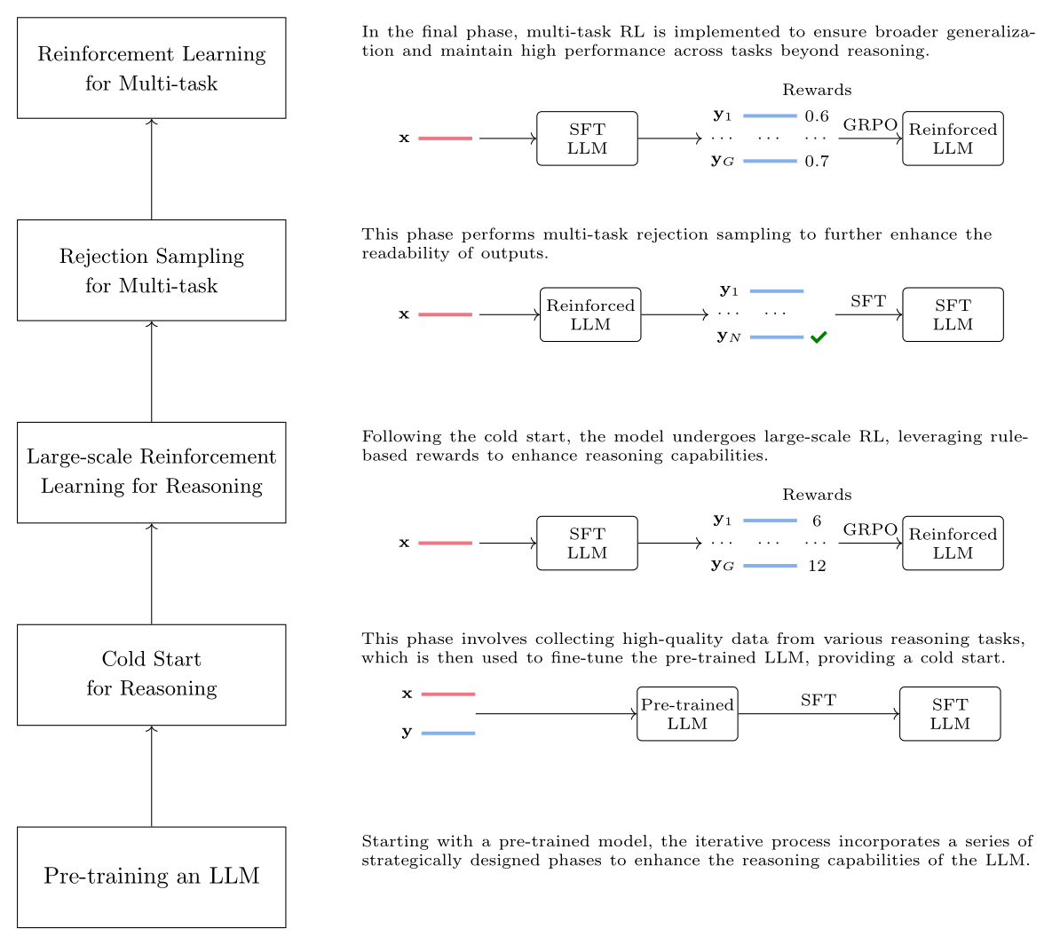
The first phase uses high-quality reasoning data as a cold start. The next phase applies large-scale RL with rule-based rewards such as format checking and answer verification to strengthen reasoning. Because this can hurt readability, rejection sampling and SFT are then used to refine outputs across multiple tasks. A final multi-task RL phase improves generalization with a broader reward model.
The order matters. Reasoning-oriented RL is placed early because later rejection sampling needs a model that can already explore meaningful reasoning trajectories. If this capability is missing, the sampled candidates are weak and the later SFT phase has little useful material to select from. After reasoning ability is strengthened, rejection sampling can improve readability, and multi-task RL can recover broader instruction-following behavior.
5.3 Large-scale RL
Large-scale Reasoning RL expands the iterative loop with many prompts, many sampled solutions, strong verifiers, and large training infrastructure. Scale can improve exploration and make sparse rewards more useful because the model has more opportunities to discover correct trajectories. However, it also increases the need for reliable rewards, stable optimization, and careful monitoring.
The central question is not only whether the model can find correct solutions, but whether RL can make the process of finding them part of the model's learned behavior. This is why Reasoning RL has become a major direction in modern LLM research.
The section also highlights two practical challenges. First, large-scale RL needs highly reliable rewards because the policy will actively search for behaviors that maximize them. Rule-based rewards are attractive in math and code because answer verification is relatively stable. Second, the reference model used to constrain policy drift can become too restrictive as the policy improves, so some methods periodically refresh the reference or otherwise balance stability with adaptability.
5.4 On-Policy Distillation
On-policy distillation is included because it occupies a useful middle ground between supervised distillation and RL-style feedback. It keeps the training states on-policy: the student first generates trajectories from its current policy, and the teacher then provides next-token distributional supervision at the states actually visited by the student.

This reduces the mismatch caused by offline distillation from teacher-generated trajectories. In the paper's RL formulation, the negative KL divergence between teacher and student distributions can be treated as a token-level reward, giving denser feedback than outcome-only supervision.
The distinction from ordinary distillation is important. Offline distillation trains the student on trajectories produced by the teacher, which may not match the states the student actually visits during its own generation. OPD instead lets the student generate first, then asks the teacher how to continue from those student-visited prefixes. This makes the supervision denser and more relevant to the student's real errors, at the cost of extra teacher forward passes during training.
Section 6
Agentic RL
Section 6 extends the same RL view from single generated answers to interactive agents. In the previous chapters, a trajectory was often a completion or a reasoning trace. For an agent, the trajectory includes observations, plans, tool calls, returned results, memory operations, and final task outcomes. This makes the sequence longer and the reward structure more complex.
The chapter moves from capabilities to infrastructure to learning signals. It first asks what an agent must be able to do, focusing on planning and tool use. It then asks what environment can expose those decisions and provide feedback. After that, it addresses credit assignment, because delayed task success must be connected back to earlier plans and actions. The final part explains how agents can reuse experience through memory, skills, and trajectory refinement.
| Agent Component | What the Paper Emphasizes | Training Signal |
|---|---|---|
| Planning | Decompose a task into subgoals and executable steps. | Trajectory success and plan quality. |
| Tool use | Select tools, format arguments, interpret observations, and stop appropriately. | Execution correctness, tool appropriateness, and cost. |
| Environment | Provide states, actions, observations, transitions, and verifiers. | Reliable state-based or task-success rewards. |
| Memory and skills | Convert experience into reusable information and behavior. | Future task success after retrieval or skill use. |
6.1 Building Agent Capabilities
The paper focuses on two basic agent capabilities because they create most of the later learning problems. Planning decomposes a task into subgoals and action steps. Tool use allows the model to interact with external systems such as search engines, APIs, code interpreters, databases, and software environments. Once these decisions appear, imitation data alone is usually not enough; the agent also needs feedback about whether its plan and tool calls actually worked.
Planning
Planning is the ability to infer the steps needed to complete a task even when the user does not specify those steps. In the tutorial's example, the agent sees an environment with a calculator and a database API, receives a babysitting-payment task, and must plan to extract numbers, compute \(12\times 50/60\), format the result, and save it through the API.
Supervised planning data can provide an initial scaffold. The data may include environment information, sampled trajectories, trajectory evaluation, and selected demonstrations. RL can then improve the policy through interaction, where the model receives feedback from actual task execution.
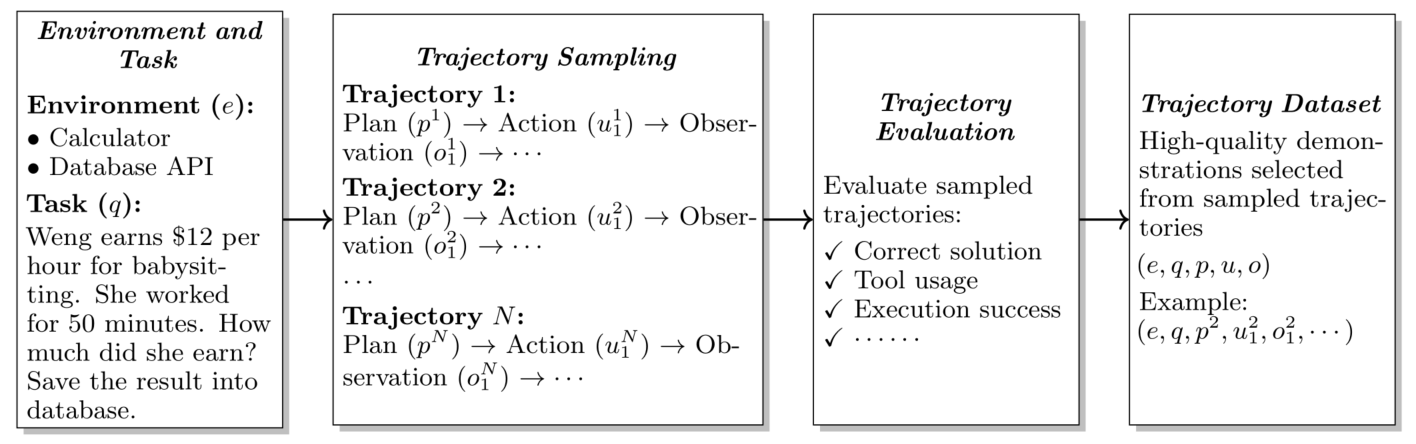
The important distinction from ordinary SFT is that a plan is judged by its downstream consequences. A locally reasonable subgoal can still lead to failure after several tool calls, while an initially failed trajectory may reveal a useful alternative. RL is useful because it can optimize plans according to execution outcomes rather than only imitate static demonstrations.
Tool Use
Tool use adds new decisions. The model must choose whether to call a tool, which tool to call, how to format the arguments, how to interpret the returned observation, and when to stop. These decisions can be optimized with rewards based on task success, execution correctness, or intermediate progress [15][16][17].
The paper presents tool learning in three levels. Prompt-based tool use gives the model tool descriptions and demonstrations, so it learns an interaction pattern in context. Supervised tool-use data fine-tunes the model on trajectories containing thoughts, actions, observations, and final answers. RL then optimizes choices that imitation alone cannot directly judge, such as whether a tool call was necessary, whether the arguments were valid, whether the observation was used correctly, and whether the cost of using the tool was justified.
| Tool-use Stage | What It Teaches | Main Limitation |
|---|---|---|
| Prompt-based tool use | How to alternate reasoning, action, observation, and answer. | Depends heavily on in-context ability. |
| Supervised tool-use data | How to imitate demonstrated tool trajectories. | Cannot directly optimize task success or tool cost. |
| RL for tool use | How to choose and execute tools based on feedback. | Requires reliable environments and rewards. |
6.2 Environment Design and Scaling
After planning and tool use, the next dependency is the environment. Environments define what an agent can learn because they specify states, available actions, transition rules, observations, and success criteria. A useful environment should be challenging enough to teach real capabilities, but structured enough to provide reliable feedback.
In Agentic RL, the environment is not just background context. It determines the action space, exposes observations after each action, and supplies the rewards or verifiers used for learning. For a tool-use task, this may include tool schemas, executable APIs, state changes, error messages, and task-success checks. Poorly designed environments can make the agent learn brittle shortcuts or receive misleading feedback.
Manual environment construction is expensive. Therefore, recent work explores synthetic and programmatic environment generation. A typical pipeline defines the environment specification, builds executable components, generates scenarios, lets the agent interact, verifies outcomes, and uses the resulting trajectories for learning [18].
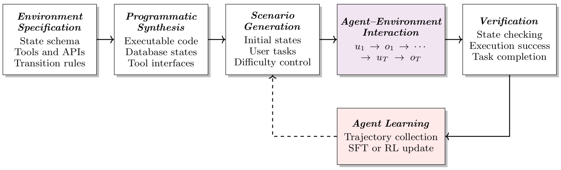
This interaction-learning loop makes agent training different from ordinary dataset training. The agent can continually encounter new tasks, expose weaknesses in its current policy, and collect trajectories that support further improvement.
6.3 Credit Assignment
Once an environment returns a final outcome, the optimizer still needs to know what to learn from it. Agent trajectories often contain many decisions before a final reward is observed. A task may fail because of an early planning error, an incorrect tool argument, a misread observation, or a wrong final answer. Credit assignment determines which parts of the trajectory should receive positive or negative learning signal.
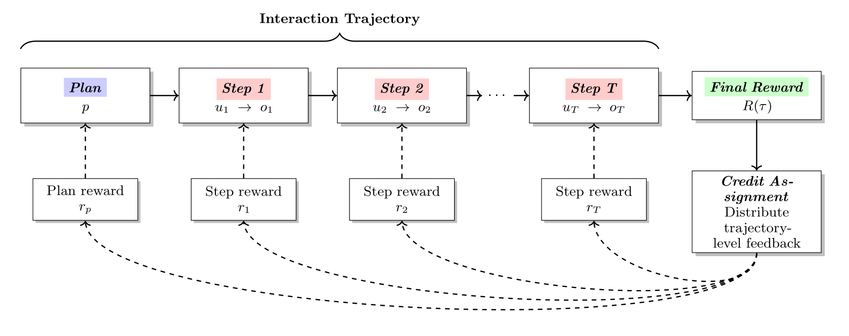
Trajectory-level rewards are often too coarse. More informative methods add intermediate rewards, process supervision, step verifiers, or models that evaluate subgoals. The goal is to connect delayed success or failure to the decisions that actually caused it [19].
The paper separates credit at different levels. Plan-level feedback evaluates whether the initial decomposition is useful. Step-level feedback evaluates individual actions such as tool calls or observation interpretation. Outcome-level feedback evaluates final task success. Combining these signals helps the agent learn not only that a trajectory failed, but which decision should be changed.
6.4 Learning from Agentic Experience
The last step is to avoid treating agent data as disposable. Agentic systems should learn not only from human demonstrations, but also from their own interaction experience. As agents operate in dynamic environments, they collect both successful and failed trajectories. These trajectories can reveal reusable knowledge, recurring solution patterns, and failure modes that are difficult to cover with static supervised data.
The paper describes this shift as moving toward agent self-evolution: the agent improves future behavior by accumulating, organizing, and reusing experience. Three mechanisms are central to this discussion: memory management stores useful information, skill optimization abstracts repeated behaviors into reusable workflows, and trajectory refinement revises agent behavior from feedback.
| Mechanism | What It Keeps From Experience | How It Improves the Agent |
|---|---|---|
| Memory management | User preferences, task facts, successful or failed trajectories. | Retrieves relevant past experience and learns which memories to add, update, delete, or ignore. |
| Skill optimization | Reusable patterns across multiple trajectories. | Turns low-level experience into high-level workflows that guide planning and tool use. |
| Trajectory refinement | Feedback from the current attempt. | Uses reflection or evaluator feedback to revise later attempts, sometimes as in-context policy improvement. |
6.4.1 Memory Management
Memory systems store useful information from past interactions and retrieve it for future tasks. A memory manager must decide what to add, update, delete, or ignore. This is a learning problem because storing too much information can introduce noise, while storing too little prevents transfer from past experience.
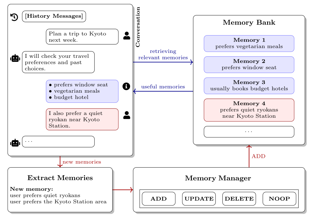
Retrieve relevant memories from the memory bank to support the current interaction.
Extract useful information from the completed interaction for future use.
Integrate new information by adding, revising, deleting, or ignoring memories.
A straightforward memory system can simply retrieve related content and store newly extracted facts. The paper emphasizes that this becomes difficult as experience accumulates: the memory bank may contain redundant, outdated, or contradictory information. A more selective system treats memory maintenance as an operation-selection problem:
These operations create a new memory, revise an existing one, remove an outdated or contradictory one, or leave the memory bank unchanged.
Recent work such as Memory-R1 turns the memory manager itself into a policy optimized by RL [25]. Given an extracted memory and the old memory bank, the manager chooses both an operation and the updated memory content:
Here, \(o\) is the selected memory operation and \(m'\) is the updated memory content. The reward can be defined by downstream task performance, for example \(R_{\mathrm{answer}}=\mathrm{EM}(y_{\mathrm{pred}},y_{\mathrm{gold}})\).
This avoids manually labeling every memory operation. If the updated memory helps the agent answer a future task correctly, the memory manager receives positive feedback; if it hurts the downstream answer, the operation is discouraged. The paper also notes a longer-horizon challenge: some memories may not be useful immediately but can help future tasks, so memory construction itself can be formulated as a sequential decision problem [26].
6.4.2 Skill Optimization
Skill optimization turns repeated successful behaviors into reusable skills. Compared with memory, which stores concrete information from past interactions, a skill is a higher-level instruction package: it can describe when to use a behavior, what workflow to follow, which tools are needed, and how to verify the final result.
During execution, the agent can be given descriptions of available skills and then select the ones most relevant to the current task. The paper writes this retrieval step as:
\(\mathcal{S}\) is the skill bank, \(\mathrm{Score}(x,s_i)\) measures relevance between the task and a skill, and \(\mathcal{S}^{*}\) is the selected skill set.
Manually writing skills can work, but the paper points out that skill quality depends heavily on human design choices. A skill that looks well structured may still fail when another agent tries to use it. SkillRL addresses this by optimizing skill generation according to whether the resulting skills improve actual agent performance [27].
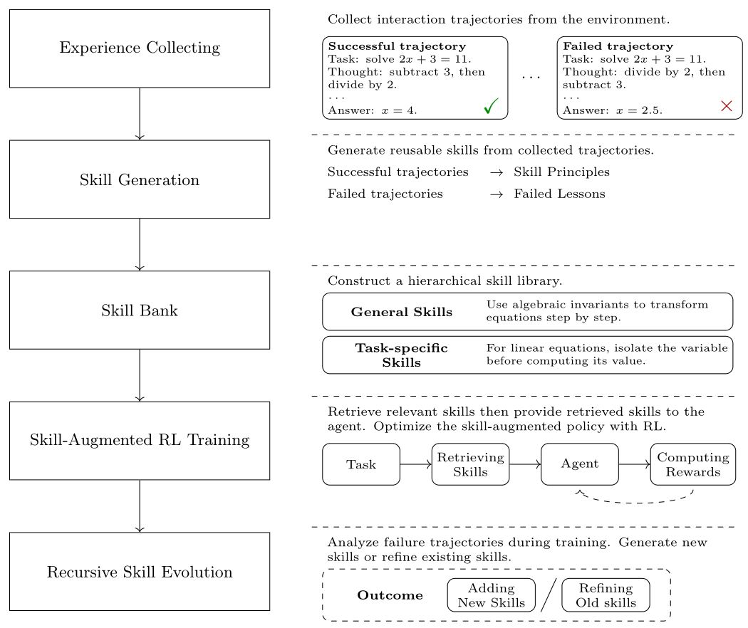
Gather successful and failed trajectories from environments.
Extract reusable skills and initialize a skill bank.
Retrieve relevant skills to guide RL exploration and planning.
Use new trajectories to discover new skills or improve old ones.
This creates a recursive loop. The skill bank gives the agent high-level behavioral priors for RL training, while the improved agent generates better trajectories that further refine the skill bank. In this sense, skill optimization compresses low-level interaction experience into reusable capabilities that can transfer across tasks.
6.4.3 Trajectory Refinement
Trajectory refinement uses feedback from an attempted solution to revise the agent's later behavior. Unlike memory management and skill optimization, which store or abstract experience for future tasks, refinement directly edits the current or next trajectory. This is especially natural for agents because tool execution results and environment states provide feedback during the interaction itself.
Start from a problem or environment goal.
Generate the first reasoning, planning, or tool-use attempt.
Receive a verifier, evaluator, tool, or environment signal.
Turn the feedback into an error analysis or improvement strategy.
Use the reflection to produce a better subsequent attempt.
Reflexion is a representative prompting-based approach: the agent produces an initial trajectory, receives evaluator feedback, writes a reflection, and uses that reflection in subsequent attempts [20]. The paper connects this to step-level feedback as well: outcome-level feedback may only say that the final answer failed, while step-level feedback can identify where the trajectory went wrong and how the agent should revise it.
Prompt-based refinement is useful, but the paper notes two limitations. First, it depends on the pretrained model's native ability to interpret feedback and revise its behavior. Second, it often helps only the current interaction, without turning failed trajectories into transferable experience. Recent work therefore trains agents to acquire refinement ability more explicitly, either through refinement tuning or exploration-based trajectory optimization [28][29].
Section 7
Multimodal RL
Section 7 extends RL beyond text-only LLMs. The reason this chapter comes after reasoning and agents is that the same abstraction must now survive a change in modality. Multimodal models process and generate information across text, images, video, and audio. The chapter separates two cases: multimodal understanding, where the model usually still generates text conditioned on non-textual inputs, and multimodal generation, where the model synthesizes images or other media.
Although the architectures differ, the core RL pattern is similar: sample outputs or generation trajectories, evaluate them with rewards, and update the model toward preferred behavior. What changes is the object being scored and the meaning of a trajectory. For visual understanding, the trajectory can still be a text answer. For image generation, the trajectory may be a denoising path or a discretized flow.
| Setting | Policy View | Reward Focus |
|---|---|---|
| Multimodal understanding | Generate answers grounded in visual or multimodal input. | Instruction following, visual faithfulness, factuality, helpfulness, and hallucination avoidance. |
| Diffusion generation | Treat the denoising process as a multi-step trajectory. | Text-image alignment, human preference, safety, or aesthetic quality. |
| Flow matching generation | Discretize a continuous generation path into decision steps. | Reward the final generated sample and optimize the generation process. |
7.1 Multimodal Understanding Models
Multimodal understanding is the closer case to LLM RL. The model must answer questions or follow instructions grounded in non-textual input, but the output is often still text. Rewards may evaluate instruction following, visual faithfulness, factual correctness, helpfulness, and hallucination avoidance. This requires reward models that understand both language and visual content [21].
From the RL perspective, visual language models are close to ordinary LLMs because the output is still usually text. The state now includes both the textual instruction and visual representations from an encoder, while the action remains the next generated token. This means PPO-style or GRPO-style training can be reused with relatively small changes, as long as the reward model can evaluate whether the text is grounded in the image.

The paper presents visual reward modeling as a natural extension of RLHF. Preference learning remains central, but the evaluated output must be judged against both the instruction and the image. This creates new challenges in data collection, model grounding, and reward generalization.
Because visual preference data is expensive, the paper describes a multi-stage strategy. First, use large-scale text preference data to pre-train general preference judgment. Second, fine-tune with image-caption preference data to reduce the task gap between general text preference and visual instruction following. Third, fine-tune with smaller visual preference data so the reward model learns the actual modality grounding needed for image-based evaluation.
This also explains why Multimodal RL is not only an algorithm problem. The policy optimizer may be familiar, but the bottleneck often lies in building a reward model that can judge visual facts, modality-specific errors, and human preferences reliably.
7.2 Multimodal Generation Models
Multimodal generation is the harder case because the output is no longer a token sequence. These models synthesize non-textual content such as images and videos, often through diffusion or continuous transformation processes. Maximum-likelihood or reconstruction-style training can learn high-quality data distributions, but it may not directly optimize high-level user preferences, such as object counts, colors, layouts, visual quality, or prompt satisfaction.
RL is useful here because the generated sample can be evaluated by flexible reward signals from humans, learned reward models, vision-language evaluators, or automatic rules. The main technical question is how to reinterpret the generation process as a trajectory so that policy-gradient-style optimization can connect the final sample reward back to the model's intermediate generation decisions.
This is why the section separately discusses diffusion models and flow matching models. They both generate non-text content, but their trajectories are different. Diffusion naturally provides a sequence of denoising states, while flow matching is often deterministic and continuous, so it needs an additional stochastic formulation before online RL can be applied.
7.2.1 Diffusion Models
Diffusion models generate samples through a gradual reverse denoising process. Starting from random noise, the model repeatedly predicts a cleaner latent until it obtains the final image. Standard diffusion training mainly teaches the model to recover the data distribution, but this does not necessarily ensure that the final sample satisfies fine-grained human requirements.
For example, a model may generate a realistic image while missing a requested object count, color, or layout. RL adds an evaluator on top of the final sample, such as a preference model or vision-language checker, and then optimizes the generation process toward samples that receive higher reward.
Here, \(\mathbf{z}\) denotes the text prompt, \(\mathbf{x}_0\) is the final generated image, and \(R_{\mathrm{dm}}(\mathbf{x}_0,\mathbf{z})\) is the reward function that evaluates whether the image satisfies the prompt or preference criteria.
The difficulty is that diffusion generation is not autoregressive token generation. Following the formulation described in the paper, the reverse denoising process can instead be viewed as a multi-step MDP. At each step, the current noisy latent and prompt form the state, and the next denoised latent is the action:
Here, \(U_{\theta}\) denotes the learned reverse denoising transition. The denoising trajectory \(\tau_{\mathrm{dm}}=\{\mathbf{x}_T,\mathbf{x}_{T-1},\ldots,\mathbf{x}_0\}\) is treated as the trajectory optimized by RL.
This follows the DPOK-style formulation in the paper: the reverse denoising process is treated as a trajectory, and the final-image reward is used to optimize the log probability of its denoising steps [22].
Under this view, the reward on the final image can be used in a policy-gradient loss over the denoising trajectory [22]. This also allows techniques from LLM alignment to transfer naturally: KL regularization can constrain the model, reference diffusion models can support importance sampling, and group-relative methods can compare multiple generated samples for the same prompt.
7.2.2 Flow Matching Models
Flow matching models generate content by learning a continuous-time flow between a simple prior distribution and the target data distribution. Instead of gradually adding and removing noise as in diffusion models, flow matching learns a velocity field that transports samples along a continuous trajectory.
This creates a different RL problem. Diffusion has stochastic denoising transitions that can be treated like policy actions. Standard flow matching often follows a deterministic ODE path once the initial noise is fixed, which limits exploration and makes transition probabilities harder to use in policy-gradient updates.
Here, \(\mathbf{x}_0\) denotes a data sample, \(\mathbf{x}_1\) denotes a noise sample, \(t\in[0,1]\) is the continuous time variable, and \(\mathbf{v}_{\theta}\) is the learned velocity field.
To apply RL, the continuous generation path can be discretized into decision steps. The state includes the prompt, time, and current sample; the action is the next state predicted by the flow model:
Here, \(\mathbf{z}\) is the text condition, \(\Delta t\) is the discretization step, and \(a_t\) denotes the next sample state produced by the generator.
A direct ODE formulation is deterministic, which creates a problem for online RL: policy-gradient methods need stochastic sampling to explore different trajectories and compute transition probabilities. Flow-GRPO addresses this by converting the deterministic flow into an equivalent stochastic differential equation that preserves the marginal distribution while injecting sampling diversity [23].
Here, \(\mu_{\theta}\) is determined by the learned velocity field, \(\sigma_t\) controls sampling stochasticity, \(R_{\mathrm{fm}}\) evaluates the final generated sample, and \(\hat{A}_i\) is computed from the relative reward of one trajectory within a sampled group.
This objective is shown under the Flow-GRPO formulation: the deterministic flow is converted into a stochastic MDP so that online RL can sample trajectories and compute transition probabilities [23].
This makes flow matching compatible with GRPO-style optimization. The model samples multiple generation trajectories for the same condition, evaluates each final sample, normalizes rewards within the group, and updates the generator according to the resulting relative advantages.
The broader message is that RL is becoming a shared optimization interface for foundation models. Once a system can produce candidate outputs and obtain evaluative feedback, many of the same design questions reappear: how to define reward, how to sample efficiently, how to assign credit, and how to avoid reward exploitation.
Section 8
Conclusions and Future Directions
The paper introduces RL from the perspective of LLM research by following one idea across increasingly rich settings: a model produces behavior, feedback evaluates that behavior, and optimization shifts the policy toward better future behavior. The early sections build the notation and PPO-style RLHF workflow. The middle sections improve the weak points of that workflow. The later sections show how the same feedback logic appears in reasoning models, agentic systems, and multimodal models.
Across these settings, RL has evolved from a general policy optimization framework into a key paradigm for enhancing LLM reasoning, interactive decision-making, and multimodal generation capabilities. At the same time, the tutorial closes by emphasizing that the field is still unsettled: rewards can be expensive or exploitable, online sampling is costly, scaling behavior is hard to predict, and continual self-improvement remains more of a research frontier than a solved recipe.
Appendix
Useful Systems and Datasets
The appendix makes the introduction practical by listing systems, datasets, and environments used in modern RL for LLMs. After the main chapters explain the concepts, this resource layer helps readers find concrete tooling and data for reward modeling, Reasoning RL, Agentic RL, and Multimodal RL post-training. Systems differ in their support for PPO, GRPO, DPO, multimodal training, asynchronous rollouts, tool calling, and agent environments. Datasets differ in feedback source, scale, modality, and target use case.
Systems
| System | Text | Image | Video | Audio | Supported Training Approaches |
|---|---|---|---|---|---|
| TRL | Yes | Yes | No | No | SFT, reward modeling, PPO, GRPO, RLOO, DPO, KTO, ORPO, Online-DPO; Agentic RL via OpenEnv/Harbor. |
| OpenRLHF | Yes | Yes | No | No | SFT, reward modeling, PPO, REINFORCE++, GRPO, RLOO, Dr.GRPO, DPO, KTO; Agentic RL with single-turn/multi-turn executors. |
| verl | Yes | Yes | No | No | SFT, PPO, GRPO, GSPO, ReMax, REINFORCE++, RLOO, DAPO, Dr.GRPO; Agentic RL via multi-turn tool calling. |
| verl-agent | Yes | Yes | No | No | GiGPO, GRPO, PPO, DAPO, GSPO, RLOO, REINFORCE++, LoRA; purpose-built Agentic RL for long-horizon LLM/VLM agents. |
| EasyR1 | Yes | Yes | No | No | GRPO, DAPO, REINFORCE++, ReMax, RLOO, GSPO, CISPO; no native Agentic RL. |
| LLaMA-Factory | Yes | Yes | Yes | Yes | Pre-training, SFT, reward modeling, PPO, DPO, KTO, ORPO, SimPO; no native Agentic RL. |
| VeOmni | Yes | Yes | Yes | Yes | Single-/multi-modal pre-training and post-training, SFT-style training, DPO, RL trainer backend; no native Agentic RL environment stack. |
| ms-swift | Yes | Yes | Yes | Yes | Pre-training, SFT, reward modeling, PPO, GRPO, DPO, KTO, ORPO, CPO, SimPO, GKD; Agentic RL via multi-turn GRPO/tool-use training. |
| Align-Anything | Yes | Yes | Yes | Yes | SFT, reward modeling, PPO, DPO, KTO, ORPO, SimPO, rule-based RL; Agentic RL on roadmap. |
| OpenRLHF-M | No | Yes | No | No | PPO, GRPO, RLOO, Online-RLHF, Rejection Sampling for multimodal models; no native Agentic RL. |
| DeepSpeed-Chat | Yes | No | No | No | SFT, reward modeling, PPO-based RLHF; no native Agentic RL. |
| ROLL | Yes | Yes | No | No | SFT, DPO, distillation, PPO, GRPO, REINFORCE++, GSPO, RAFT++, StarPO, GiGPO; Agentic RL. |
| slime | Yes | No | No | No | PPO, GRPO, GSPO, REINFORCE++, OPD; Agentic RL via custom generation, tools, sandboxes, and verifier rewards. |
| OpenClaw-RL | Yes | Yes | No | No | Binary RL/GRPO, OPD, Hybrid RL, LoRA training; asynchronous Agentic RL for personalized agents, terminal, GUI, SWE, and tool-call settings. |
| SkyRL | Yes | No | No | No | GRPO, DAPO, async RL, Tinker-compatible training; Agentic RL for tool-use, search, SQL, and long-horizon tasks. |
| Agent Lightning | Yes | No | No | No | RL, APO, SFT-style optimization hooks; purpose-built Agentic RL for existing agent frameworks. |
| RAGEN | Yes | No | No | No | PPO/StarPO-style multi-turn optimization, environment rewards; Agentic RL. |
| Search-R1 | Yes | No | No | No | PPO, GRPO, REINFORCE for reasoning-search interleaved models; Agentic RL for search/tool use. |
| AReaL | Yes | No | No | No | PPO/GRPO-style RL with agent-framework integration; Agentic RL. |
Datasets
| Dataset | Reward Model | Reasoning | Agent | Scale | Modality | Source | Category |
|---|---|---|---|---|---|---|---|
| Anthropic/hh-rlhf | Yes | No | No | 169K | Text | Human | Pairwise preference |
| stanfordnlp/SHP-2 | Yes | No | No | 4.8M | Text | Human / crowd | Pairwise preference |
| H4/stack-exchange-preferences | Yes | No | No | 10.7M | Text | Crowd score | Score / ranking |
| Summarize from Feedback | Yes | No | No | 64.8K | Text | Human | Pairwise preference |
| UltraFeedback | Yes | No | No | 64K / 340K | Text | GPT-4 | Scores, critiques, pairs |
| berkeley-nest/Nectar | Yes | No | No | 183K / 3.8M | Text | GPT-4 | 7-way ranking |
| Skywork-Reward-Preference-80K | Yes | No | No | 80K | Text | Mixed / curated | Pairwise preference |
| nvidia/HelpSteer | Yes | No | No | 37K | Text | Human | Attribute scores |
| nvidia/HelpSteer2 | Yes | No | No | 10K pairs | Text | Human | Attribute scores / preference |
| nvidia/HelpSteer3 | Yes | No | No | 40K pref. | Text | Human | Preference, feedback, edits |
| Arena Human Preference 55K | Yes | No | No | 55K | Text | Human users | Arena battle preference |
| VLFeedback | Yes | No | No | 80K / 380K | Text, Image | GPT-4V | Multimodal preference |
| RLHF-V-Dataset | Yes | No | No | 5.7K | Text, Image | Human | Fine-grained correction |
| openbmb/RLAIF-V-Dataset | Yes | No | No | 83K | Text, Image | AI feedback | Pairwise preference |
| OpenGVLab/MMPR-v1.2 | Yes | Yes | No | 3M | Text, Image | AI / verifier | Multimodal reasoning preference |
| open-r1/OpenR1-Math-220k | No | Yes | No | 220K | Text | Verifier / judge | Math reasoning traces |
| AI-MO/NuminaMath | No | Yes | No | 900K | Text | Rule / GPT-4 | Math CoT / TIR |
| PRIME-RL/Eurus-2-RL-Data | No | Yes | No | 482K | Text | Verifier | Math/code outcome reward |
| AgentGym-RL-Data | No | Yes | Yes | 184K | Text | Environment | Multi-turn agent reward |
| ALFWorld | No | No | Yes | 3.5K train | Text | Environment | Text-world task reward |
| WebShop | No | No | Yes | 12K tasks | Text | Environment | Web shopping reward |
| Search-R1 Data | No | Yes | Yes | 170K train | Text | Retriever / rule | Search-tool QA reward |
| Sokoban | No | Yes | Yes | Environment-generated | Text, Image | Environment | Puzzle-solving reward |
| Gym Cards | No | Yes | Yes | Environment-generated | Text, Image | Environment | Logic-game reward |
| ToolBench | No | Yes | Yes | 126K | Text | API execution | Tool-use trajectories |
This resource layer complements the main introduction with concrete systems and datasets. Because new methods and systems appear rapidly, especially around Reasoning RL, Agentic RL, and Multimodal RL post-training, the website provides a compact entry point into the surrounding ecosystem.
Note: the systems table was compiled in August 2026. Some systems may have changed after publication; if current releases differ from the table, please contact the authors so the information can be updated.
Selected sources
References
- Richard S. Sutton and Andrew G. Barto. Reinforcement Learning: An Introduction (2nd ed.). The MIT Press, 2018.
- Long Ouyang, Jeffrey Wu, Xu Jiang, Diogo Almeida, Carroll L. Wainwright, Pamela Mishkin, Chong Zhang, Sandhini Agarwal, Katarina Slama, Alex Ray, John Schulman, Jacob Hilton, Fraser Kelton, Luke Miller, Maddie Simens, Amanda Askell, Peter Welinder, Paul F. Christiano, Jan Leike, and Ryan Lowe. Training language models to follow instructions with human feedback. NeurIPS 2022, 2022.
- Paul F. Christiano, Jan Leike, Tom B. Brown, Miljan Martic, Shane Legg, and Dario Amodei. Deep reinforcement learning from human preferences. NeurIPS 2017, 2017.
- John Schulman, Filip Wolski, Prafulla Dhariwal, Alec Radford, and Oleg Klimov. Proximal policy optimization algorithms, 2017.
- Ralph Allan Bradley and Milton E. Terry. Rank analysis of incomplete block designs: I. the method of paired comparisons. Biometrika, 1952.
- Dakota Mahan, Duy Van Phung, Rafael Rafailov, Chase Blagden, Nathan Lile, Louis Castricato, Jan-Philipp Franken, Chelsea Finn, and Alon Albalak. Generative reward models, 2024.
- Tianci Liu, Ran Xu, Tony Yu, Ilgee Hong, Carl Yang, Tuo Zhao, and Haoyu Wang. OpenRubrics: Towards scalable synthetic rubric generation for reward modeling and LLM alignment. ACL 2026, 2026.
- Nathan Lambert, Valentina Pyatkin, Jacob Morrison, LJ Miranda, Bill Yuchen Lin, Khyathi Chandu, Nouha Dziri, Sachin Kumar, Tom Zick, Yejin Choi, Noah A. Smith, and Hannaneh Hajishirzi. RewardBench: Evaluating reward models for language modeling. Findings of NAACL 2025, 2025.
- John Schulman, Philipp Moritz, Sergey Levine, Michael I. Jordan, and Pieter Abbeel. High-dimensional continuous control using generalized advantage estimation. ICLR 2016, 2016.
- Zhihong Shao, Peiyi Wang, Qihao Zhu, Runxin Xu, Junxiao Song, Xiao Bi, Haowei Zhang, Mingchuan Zhang, YK Li, Y Wu, et al. DeepSeekMath: Pushing the limits of mathematical reasoning in open language models, 2024.
- Rafael Rafailov, Archit Sharma, Eric Mitchell, Christopher D. Manning, Stefano Ermon, and Chelsea Finn. Direct preference optimization: Your language model is secretly a reward model. NeurIPS 2023, 2023.
- DeepSeek. DeepSeek-R1: Incentivizing reasoning capability in LLMs via reinforcement learning, 2025.
- Hunter Lightman, Vineet Kosaraju, Yuri Burda, Harrison Edwards, Bowen Baker, Teddy Lee, Jan Leike, John Schulman, Ilya Sutskever, and Karl Cobbe. Let's verify step by step. ICLR 2024, 2024.
- David Silver, Julian Schrittwieser, Karen Simonyan, Ioannis Antonoglou, Aja Huang, Arthur Guez, Thomas Hubert, Lucas Baker, Matthew Lai, Adrian Bolton, et al. Mastering the game of Go without human knowledge. Nature, 2017.
- Shunyu Yao, Jeffrey Zhao, Dian Yu, Nan Du, Izhak Shafran, Karthik R. Narasimhan, and Yuan Cao. ReAct: Synergizing reasoning and acting in language models. ICLR 2023, 2023.
- Timo Schick, Jane Dwivedi-Yu, Roberto Dessi, Roberta Raileanu, Maria Lomeli, Eric Hambro, Luke Zettlemoyer, Nicola Cancedda, and Thomas Scialom. Toolformer: Language models can teach themselves to use tools. NeurIPS 2023, 2023.
- Cheng Qian, Emre Can Acikgoz, Qi He, Hongru Wang, Xiusi Chen, Dilek Hakkani-Tur, Gokhan Tur, and Heng Ji. ToolRL: Reward is all tool learning needs. NeurIPS 2025, 2025.
- Mengkang Hu, Pu Zhao, Can Xu, Qingfeng Sun, Jian-Guang Lou, Qingwei Lin, Ping Luo, and Saravan Rajmohan. AgentGen: Enhancing planning abilities for large language model based agent via environment and task generation. KDD 2025, 2025.
- Zhiwei Li, Yong Hu, and Wenqing Wang. Encouraging good processes without the need for good answers: Reinforcement learning for LLM agent planning. EMNLP Industry Track 2025, 2025.
- Noah Shinn, Federico Cassano, Ashwin Gopinath, Karthik Narasimhan, and Shunyu Yao. Reflexion: language agents with verbal reinforcement learning. NeurIPS 2023, 2023.
- Zhiqing Sun, Sheng Shen, Shengcao Cao, Haotian Liu, Chunyuan Li, Yikang Shen, Chuang Gan, Liangyan Gui, Yu-Xiong Wang, Yiming Yang, Kurt Keutzer, and Trevor Darrell. Aligning large multimodal models with factually augmented RLHF. Findings of ACL 2024, 2024.
- Ying Fan, Olivia Watkins, Yuqing Du, Hao Liu, Moonkyung Ryu, Craig Boutilier, Pieter Abbeel, Mohammad Ghavamzadeh, Kangwook Lee, and Kimin Lee. DPOK: Reinforcement learning for fine-tuning text-to-image diffusion models. NeurIPS 2023, 2023.
- Jie Liu, Gongye Liu, Jiajun Liang, Yangguang Li, Jiaheng Liu, Xintao Wang, Pengfei Wan, Di Zhang, and Wanli Ouyang. Flow-GRPO: Training flow matching models via online RL. NeurIPS 2025, 2025.
- David Silver, Satinder Singh, Doina Precup, and Richard S. Sutton. Reward is enough. Artificial Intelligence, 2021.
- Sikuan Yan, Xiufeng Yang, Zuchao Huang, Ercong Nie, Zifeng Ding, Zonggen Li, Xiaowen Ma, Jinhe Bi, Kristian Kersting, Jeff Z. Pan, Hinrich Schuetze, Volker Tresp, and Yunpu Ma. Memory-R1: Enhancing large language model agents to manage and utilize memories via reinforcement learning. ACL 2026, 2026.
- Yu Wang, Ryuichi Takanobu, Zhiqi Liang, Yuzhen Mao, Yuanzhe Hu, Julian McAuley, and Xiaojian Wu. Mem-alpha: Learning memory construction via reinforcement learning, 2025.
- Peng Xia, Jianwen Chen, Hanyang Wang, Jiaqi Liu, Kaide Zeng, Yu Wang, Siwei Han, Yiyang Zhou, Xujiang Zhao, Haifeng Chen, et al. SkillRL: Evolving agents via recursive skill-augmented reinforcement learning, 2026.
- Dayuan Fu, Keqing He, Yejie Wang, Wentao Hong, Zhuoma Gongque, Weihao Zeng, Wei Wang, Jingang Wang, Xunliang Cai, and Weiran Xu. AgentRefine: Enhancing agent generalization through refinement tuning. ICLR 2025, 2025.
- Yifan Song, Da Yin, Xiang Yue, Jie Huang, Sujian Li, and Bill Yuchen Lin. Trial and error: Exploration-based trajectory optimization of LLM agents. ACL 2024, 2024.